Diagnosing the Meridional Overturning Circulation on a tripolar grid with sectionate

Import packages

import numpy as np
import xgcm
import xarray as xr
import matplotlib.pyplot as plt
from dask.diagnostics import ProgressBar

import sectionate
print(f"Sectionate version: {sectionate.__version__}")

Sectionate version: 0.3.3

Load example model grid and transport diagnosics

from load_example_model_grid import load_MOM6_example_grid
grid = load_MOM6_example_grid()
ds = grid._ds

Diagnosing Meridional Overturning Streamfunctions

Density vs. Nominal Latitude Overturning

It is straight-forward to calculate the nominal-MOC (along the grid’s nominal latitude coordinate y) by integrating Y-face velocities X and Z.

rho0 = 1035. # kg/m3
Sv_s_per_m3 = 1e-6
Sv_s_per_kg = Sv_s_per_m3/rho0

%time moc_nominal = ds.vmo.cumsum("sigma2_l").sum("xh").compute() * Sv_s_per_kg

CPU times: user 22.3 ms, sys: 21.7 ms, total: 44 ms
Wall time: 49.2 ms

moc_nominal.mean('time').plot(x="yq", y="rho2_l", vmin=-30, vmax=30, cmap="RdBu_r")
plt.ylim(1038, 1028);

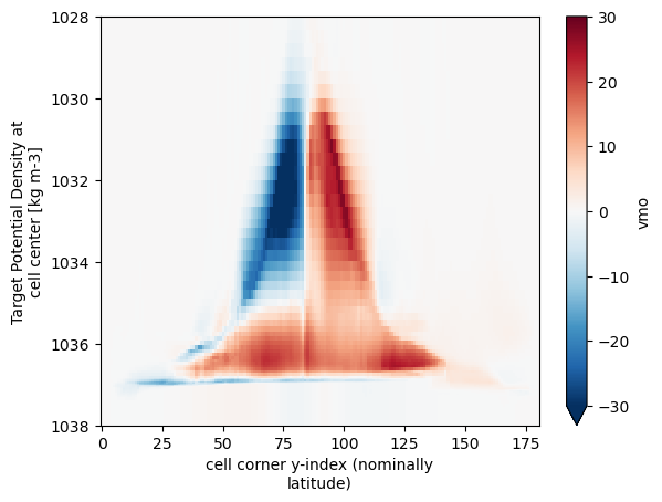
However, this is not actually the true latitudinal-MOC, which would be aligned with the geolat coordinate.

Density vs. Latitude Overturning

Using sectionate, we can compute the true northward transports across each latitude band and use these to compute the true latitudinal-MOC:

def transport_across_latitude_line(grid, lat, dlon=5.):
    section_lons=np.arange(0., 360.+dlon, dlon)
    section_lats=[lat]*len(section_lons)
    i_c, j_c, lons_c, lats_c = sectionate.grid_section(
        grid,
        section_lons,
        section_lats,
        topology="MOM-tripolar"
    )
    conv_transport = sectionate.convergent_transport(grid, i_c, j_c, layer="sigma2_l", interface="sigma2_i")
    northward_transport = -conv_transport['conv_mass_transport'].cumsum("sigma2_l").sum("sect")

    return northward_transport.expand_dims({'lat': xr.DataArray([lat], dims=('lat',))})

def global_moc(grid, dlat=2.):
    return xr.concat([transport_across_latitude_line(grid, lat) for lat in np.arange(-76, 89., dlat)], dim="lat")

Note: This operation takes a long time because of the many calls to infer_grid_path within sectionate, which is not presently vectorized. Once the section indices are computed however, the actually extraction of transports from the mass transport diagnostics takes no longer than the alternative of sum('xh'). Alternatively, sectionate’s sibling package regionate can be used used to more directly infer sections from the boundaries of Boolean masks (e.g. ds.geolat < lat).

dlat = 2
%time moc = global_moc(grid, dlat=dlat).compute() * Sv_s_per_kg

/Users/hfdrake/code/sectionate/sectionate/section.py:726: RuntimeWarning: invalid value encountered in scalar divide
  return np.arccos(np.clip((np.cos(a) - np.cos(b)*np.cos(c))/(np.sin(b)*np.sin(c)), -1., 1.))

CPU times: user 34.8 s, sys: 1.65 s, total: 36.5 s
Wall time: 37.2 s

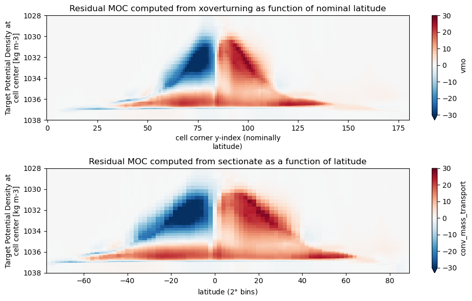
Difference between the nominal-MOC (along the yh coordinate) and the latitudinal-MOC (along the geolat coordinate)

plt.figure(figsize=(10, 6))

plt.subplot(2,1,1)
moc_nominal.mean('time').plot(x="yq", y="rho2_l", vmin=-30, vmax=30., cmap="RdBu_r")
plt.ylim(1038, 1028)
plt.title("Residual MOC computed from xoverturning as function of nominal latitude")

plt.subplot(2,1,2)
moc.mean('time').plot(x="lat", y="rho2_l", vmin=-30, vmax=30., cmap="RdBu_r")
plt.ylim(1038, 1028)
plt.xlabel(fr"latitude ({dlat}$\degree$ bins)");
plt.title("Residual MOC computed from sectionate as a function of latitude")
plt.tight_layout();