Testing the limits of `sectionate` with various edge cases¶

Can sectionate handle the curvilinear geometry and complicated topology of the tripolar configuration of MOM? Yes.

This notebook demonstrates its correct behavior in a number of non-trivial edge cases in which sections cross grid boundaries.

Import packages¶

[1]:

import xgcm
import xarray as xr
import numpy as np
import matplotlib.pylab as plt
import matplotlib.path as mpath

import cartopy.crs as ccrs
import cartopy.feature as cfeature
subplot_kws=dict(projection=ccrs.Robinson())
data_crs = ccrs.PlateCarree()

import sectionate
print(f"Sectionate version: {sectionate.__version__}")

Sectionate version: 0.3.3

Define plotting functions¶

[2]:

cmap = plt.get_cmap("Blues").copy()
cmap.set_bad((0.8, 0.8, 0.8))

def plot_sections(i_c, j_c, lons_c, lats_c, section_lons, section_lats, ds, projection=ccrs.Robinson(), vlim=[0, 7500]):

    fig, axes = plt.subplots(1, 2, figsize=[16,6], subplot_kw={'projection':projection})
    ax = axes[0]
    ds['deptho'].plot(x='geolon', y='geolat', ax=ax, transform=data_crs, cmap=plt.get_cmap("Blues"), vmin=vlim[0], vmax=vlim[1])
    ds['deptho'].plot.contour(x='geolon', y='geolat', ax=ax, transform=data_crs, colors="k", linewidths=0.5, linestyles="solid", levels=[1.])
    ax.plot(lons_c, lats_c, 'k.-', transform=ccrs.Geodetic(), markersize=1.5, lw=0.5)
    ax.plot(section_lons, section_lats, "C3x", transform=data_crs, markersize=6., mew=3., alpha=0.85, label="Points of target section")
    ax.plot([60,60], [-75, 90], "w--", alpha=0.75, lw=1.75, transform=ccrs.Geodetic(), label="nominal ds boundary")
    ax.set_xlabel("longitude")
    ax.set_ylabel("latitude")
    ax.set_title("With respect to geographic coordinates")
    ax.legend(loc="upper right", fontsize=12, labelspacing=0.12)
    ax.gridlines(alpha=0.2)
    ax.set_extent([-180, 180., -80, 80], ccrs.PlateCarree())

    if projection==ccrs.SouthPolarStereo():
        ax.set_extent([0, 360., -90, -40], ccrs.PlateCarree())

        # Compute a circle in axes coordinates, which we can use as a boundary
        # for the map. We can pan/zoom as much as we like - the boundary will be
        # permanently circular.
        theta = np.linspace(0, 2*np.pi, 100)
        center, radius = [0.5, 0.5], 0.5
        verts = np.vstack([np.sin(theta), np.cos(theta)]).T
        circle = mpath.Path(verts * radius + center)

        ax.set_boundary(circle, transform=ax.transAxes)

    elif projection==ccrs.NorthPolarStereo():
        ax.set_extent([0, 360., 50, 90], ccrs.PlateCarree())

        # Compute a circle in axes coordinates, which we can use as a boundary
        # for the map. We can pan/zoom as much as we like - the boundary will be
        # permanently circular.
        theta = np.linspace(0, 2*np.pi, 100)
        center, radius = [0.5, 0.5], 0.5
        verts = np.vstack([np.sin(theta), np.cos(theta)]).T
        circle = mpath.Path(verts * radius + center)

        ax.set_boundary(circle, transform=ax.transAxes)

    ax = axes[1]
    ax = plt.subplot(1,2,2)
    pc = ax.pcolormesh(ds['deptho'].values, cmap=cmap, vmin=vlim[0], vmax=vlim[1])
    ax.contour(ds['deptho'].values, colors="k", linewidths=0.5, linestyles="solid", levels=[1.])
    ax.plot(i_c, j_c, 'k.', markersize=1.5)
    ax.set_title("With respect to model indices (i_c,j_c)");
    plt.colorbar(pc, ax=ax)
    plt.tight_layout()

    return fig, axes

Load the model grid¶

[3]:

from load_example_model_grid import load_MOM6_example_grid
grid = load_MOM6_example_grid()
ds = grid._ds

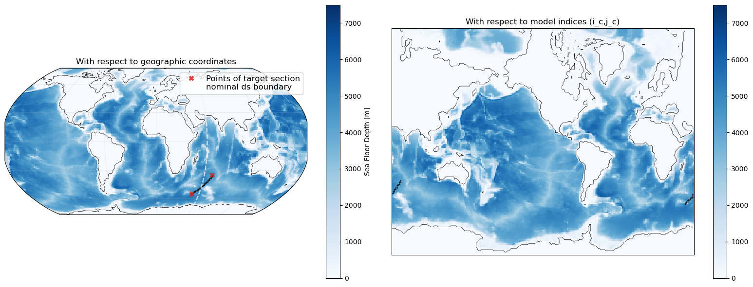
1. A section that crosses the periodic `X` boundary¶

[4]:

section_lons=[50, 70]
section_lats=[-55, -35]

assert section_lons[0] < ds['geolon_c'].max().values < section_lons[1]

Desired behavior with `boundary={"X":"periodic"}` (new default)¶

[5]:

i_c, j_c, lons_c, lats_c = sectionate.create_section_composite(
    grid._ds['geolon_c'],
    grid._ds['geolat_c'],
    section_lons,
    section_lats,
    sectionate.check_symmetric(grid),
    boundary={"X":"periodic"},
    topology="MOM-tripolar"
)

plot_sections(i_c, j_c, lons_c, lats_c, section_lons, section_lats, ds);

../_images/examples_4_sections_on_global_tripolar_grid_10_0.png

The grid_section function uses the xgcm.Grid instance to pass the correct arguments for symmetric and boundary to create_section_composite.

[6]:

i_c, j_c, lons_c, lats_c = sectionate.grid_section(
    grid,
    section_lons,
    section_lats,
    topology="MOM-tripolar"
)

plot_sections(i_c, j_c, lons_c, lats_c, section_lons, section_lats, ds);

../_images/examples_4_sections_on_global_tripolar_grid_12_0.png

2. Zonally-periodic sections¶

Note: Sectionate requires intermediate points to disambiguate zonal sections longer than 180º.

Consider the case below where we aim to make a zonally-circumpolar section that passes through Drake Passage at 60ºS.

[7]:

lat = -57.5

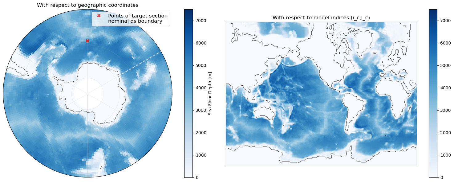
Incorrect use: no intermediate points \(\rightarrow\) no section required to connect consecutive points¶

[8]:

section_lons=[0, 360]
section_lats=[lat]*len(section_lons)

i_c, j_c, lons_c, lats_c = sectionate.grid_section(
    grid,
    section_lons,
    section_lats,
    topology="MOM-tripolar"
)
plot_sections(i_c, j_c, lons_c, lats_c, section_lons, section_lats, ds, projection=ccrs.SouthPolarStereo());

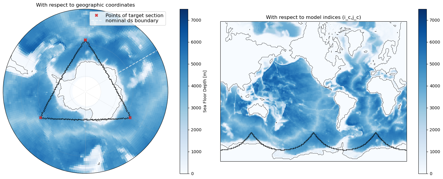
../_images/examples_4_sections_on_global_tripolar_grid_18_0.png

Incorrect use: intermediate points more than 180º apart \(\rightarrow\) shortest subsections do not cirumnavigate (and just go out and back)¶

[9]:

section_lons=[0, 240, 360]
section_lats=[lat]*len(section_lons)

i_c, j_c, lons_c, lats_c = sectionate.grid_section(
    grid,
    section_lons,
    section_lats,
    topology="MOM-tripolar"
)
plot_sections(i_c, j_c, lons_c, lats_c, section_lons, section_lats, ds, projection=ccrs.SouthPolarStereo());

../_images/examples_4_sections_on_global_tripolar_grid_20_0.png

Correct use: series of intermediate points less than 180º apart¶

[10]:

dlon=120
section_lons=np.arange(0., 360.+dlon, dlon)
section_lats=[lat]*len(section_lons)

i_c, j_c, lons_c, lats_c = sectionate.grid_section(
    grid,
    section_lons,
    section_lats,
    topology="MOM-tripolar"
)

plot_sections(i_c, j_c, lons_c, lats_c, section_lons, section_lats, ds, projection=ccrs.SouthPolarStereo());

../_images/examples_4_sections_on_global_tripolar_grid_22_0.png

To make strictly zonal sections, simply stitch together many great circle arcs:

[11]:

dlon=5
section_lons=np.arange(0., 360.+dlon, dlon)
section_lats=[lat]*len(section_lons)

i_c, j_c, lons_c, lats_c = sectionate.grid_section(
    grid,
    section_lons,
    section_lats,
    topology="MOM-tripolar"
)
plot_sections(i_c, j_c, lons_c, lats_c, section_lons, section_lats, ds, projection=ccrs.SouthPolarStereo());

../_images/examples_4_sections_on_global_tripolar_grid_24_0.png

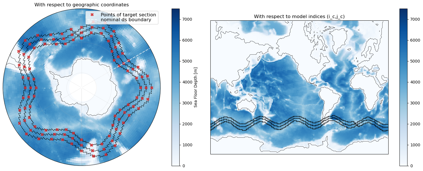
3. Example of a complex section that crosses the boundary multiple times¶

[12]:

section_lons= np.arange(0, 360*3, 10.)
section_lats= lat + section_lons*(10/3.)/360. + 5*np.sin(5* (2*np.pi*section_lons/360.))

section_lons = np.append(section_lons, section_lons[0])
section_lats = np.append(section_lats, section_lats[0])

i_c, j_c, lons_c, lats_c = sectionate.grid_section(
    grid,
    section_lons,
    section_lats,
    topology="MOM-tripolar"
)
plot_sections(i_c, j_c, lons_c, lats_c, section_lons, section_lats, ds, projection=ccrs.SouthPolarStereo());

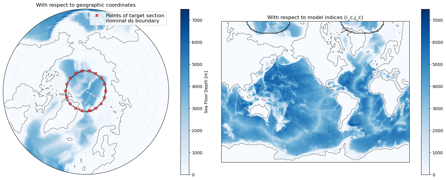
../_images/examples_4_sections_on_global_tripolar_grid_26_0.png

4. Verify that sections work correctly near and across MOM6’s tripolar grid seams¶

[13]:

section_lons=[0, 120, 240, 360]
section_lats=[80]*len(section_lons)

i_c, j_c, lons_c, lats_c = sectionate.grid_section(
    grid,
    section_lons,
    section_lats,
    topology="MOM-tripolar"
)
plot_sections(i_c, j_c, lons_c, lats_c, section_lons, section_lats, ds, projection=ccrs.NorthPolarStereo());

../_images/examples_4_sections_on_global_tripolar_grid_28_0.png

[14]:

section_lons=[0, 120, 240, 360]
section_lats=[70]*len(section_lons)

i_c, j_c, lons_c, lats_c = sectionate.grid_section(
    grid,
    section_lons,
    section_lats,
    topology="MOM-tripolar"
)
plot_sections(i_c, j_c, lons_c, lats_c, section_lons, section_lats, ds, projection=ccrs.NorthPolarStereo());

../_images/examples_4_sections_on_global_tripolar_grid_29_0.png

[15]:

dlon = 20.
section_lons=np.arange(dlon/2, 360.+dlon, dlon)
section_lats=[80]*len(section_lons)

i_c, j_c, lons_c, lats_c = sectionate.grid_section(
    grid,
    section_lons,
    section_lats,
    topology="MOM-tripolar"
)
plot_sections(i_c, j_c, lons_c, lats_c, section_lons, section_lats, ds, projection=ccrs.NorthPolarStereo());

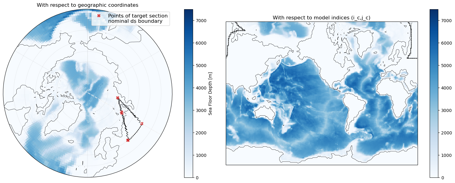
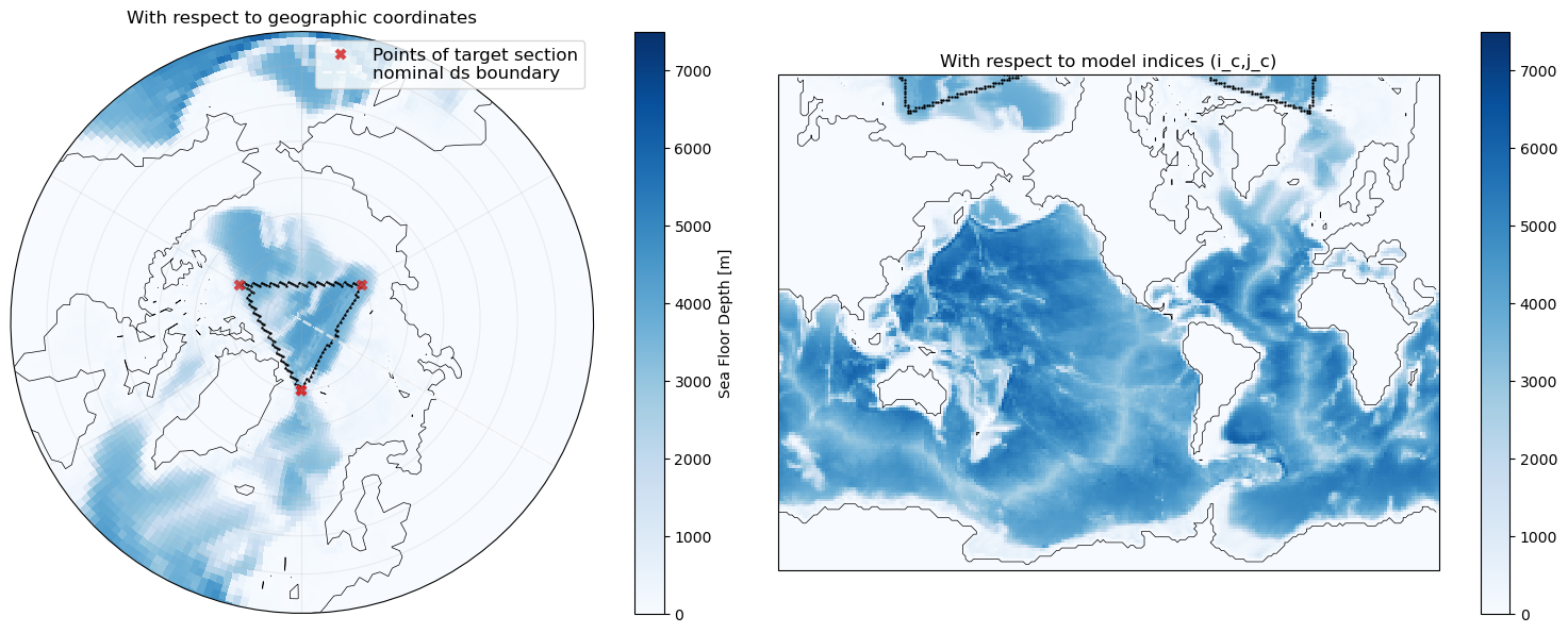
../_images/examples_4_sections_on_global_tripolar_grid_30_0.png

Caution: sectionate has some difficulty when dealing with paths that traverse through the tripolar seams, apparently because it has to temporarily move backwards (go farther away from the target point) in order to make forward progress.

[16]:

section_lons=[40, 60, 80., 40]
section_lats=[60, 60, 75, 60]

i_c, j_c, lons_c, lats_c = sectionate.grid_section(
    grid,
    section_lons,
    section_lats,
    topology="MOM-tripolar"
)
plot_sections(i_c, j_c, lons_c, lats_c, section_lons, section_lats, ds, projection=ccrs.NorthPolarStereo());

../_images/examples_4_sections_on_global_tripolar_grid_32_0.png

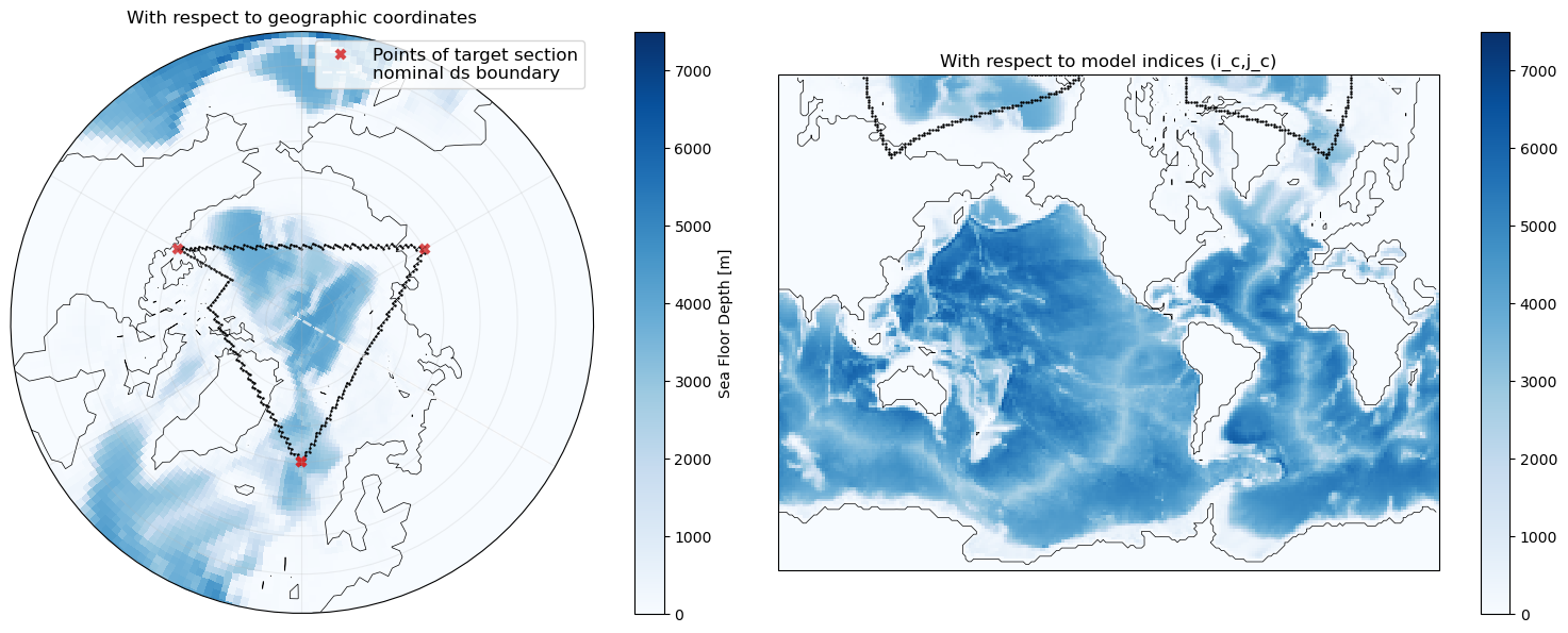
A workaround for this issue is to simply place two new points on either side of the bipolar fold right where it intersects the problematic section.

[17]:

section_lons=[40, 60, 80., 60., 59, 40]
section_lats=[60, 60, 75, 71, 70.5, 60]

i_c, j_c, lons_c, lats_c = sectionate.grid_section(
    grid,
    section_lons,
    section_lats,
    topology="MOM-tripolar"
)
plot_sections(i_c, j_c, lons_c, lats_c, section_lons, section_lats, ds, projection=ccrs.NorthPolarStereo());

../_images/examples_4_sections_on_global_tripolar_grid_34_0.png

Testing the limits of `sectionate` with various edge cases¶

Import packages¶

Define plotting functions¶

Load the model grid¶

1. A section that crosses the periodic `X` boundary¶

Desired behavior with `boundary={"X":"periodic"}` (new default)¶

2. Zonally-periodic sections¶

Incorrect use: no intermediate points \(\rightarrow\) no section required to connect consecutive points¶

Incorrect use: intermediate points more than 180º apart \(\rightarrow\) shortest subsections do not cirumnavigate (and just go out and back)¶

Correct use: series of intermediate points less than 180º apart¶

3. Example of a complex section that crosses the boundary multiple times¶

4. Verify that sections work correctly near and across MOM6’s tripolar grid seams¶

sectionate

Navigation

Related Topics

Testing the limits of sectionate with various edge cases¶

Import packages¶

Define plotting functions¶

Load the model grid¶

1. A section that crosses the periodic X boundary¶

Desired behavior with boundary={"X":"periodic"} (new default)¶

2. Zonally-periodic sections¶

Incorrect use: no intermediate points \(\rightarrow\) no section required to connect consecutive points¶

Incorrect use: intermediate points more than 180º apart \(\rightarrow\) shortest subsections do not cirumnavigate (and just go out and back)¶

Correct use: series of intermediate points less than 180º apart¶

3. Example of a complex section that crosses the boundary multiple times¶

4. Verify that sections work correctly near and across MOM6’s tripolar grid seams¶

Testing the limits of `sectionate` with various edge cases¶

1. A section that crosses the periodic `X` boundary¶

Desired behavior with `boundary={"X":"periodic"}` (new default)¶