Conservatively diagnosing model transports across arbitrary sections with sectionate
Import packages
[1]:
import numpy as np
import xgcm
import xarray as xr
import matplotlib.pyplot as plt

import sectionate
print(f"Sectionate version: {sectionate.__version__}")
Sectionate version: 0.3.3
Load example model grid and transport diagnosics
[2]:
from load_example_model_grid import load_MOM6_example_grid
grid = load_MOM6_example_grid()
ds = grid._ds
Define the two OSNAP sections:
[3]:
west_section_lats = [52.0166, 52.6648, 53.5577, 58.8944, 60.4000]
west_section_lons = [-56.8775, -52.0956, -49.8604, -47.6107, -44.8000]

east_section_lats = [60.4000, 58.8600, 58.0500, 58.0000, 56.5000]
east_section_lons = [-44.8000, -30.5400, -28.0000, -14.7000, -5.9300]

total_section_lats = west_section_lats + east_section_lats
total_section_lons = west_section_lons + east_section_lons
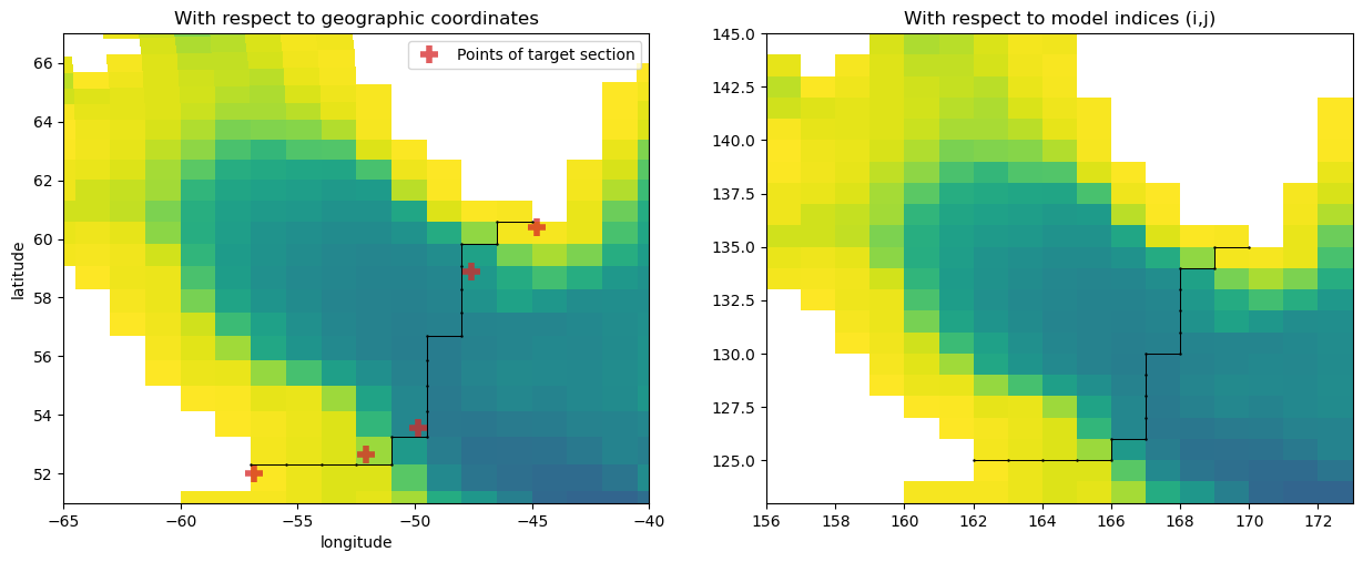
West section
[4]:
i_c, j_c, lons_c, lats_c = sectionate.grid_section(
    grid,
    west_section_lons,
    west_section_lats,
    topology="MOM-tripolar"
)
[5]:
plt.figure(figsize=[15,5.5])
plt.subplot(1,2,1)
plt.pcolormesh(ds['geolon_c'], ds['geolat_c'], ds['deptho'].where(ds['deptho']!=0), cmap="viridis_r")
plt.plot(west_section_lons, west_section_lats, "C3+", markersize=12., mew=4., alpha=0.75, label="Points of target section")
plt.plot(lons_c, lats_c, 'k.-', markersize=1.5, lw=0.75)
plt.axis([-65,-40, 51, 67])
plt.xlabel("longitude")
plt.ylabel("latitude")
plt.title("With respect to geographic coordinates")
plt.legend(loc="upper right")

plt.subplot(1,2,2)
plt.pcolormesh(ds['deptho'].where(ds['deptho']!=0).values, cmap="viridis_r")
plt.plot(i_c, j_c, 'k.-', markersize=1.5, lw=0.75)
plt.axis([156, 173, 123, 145])
plt.title("With respect to model indices (i,j)")
plt.show()
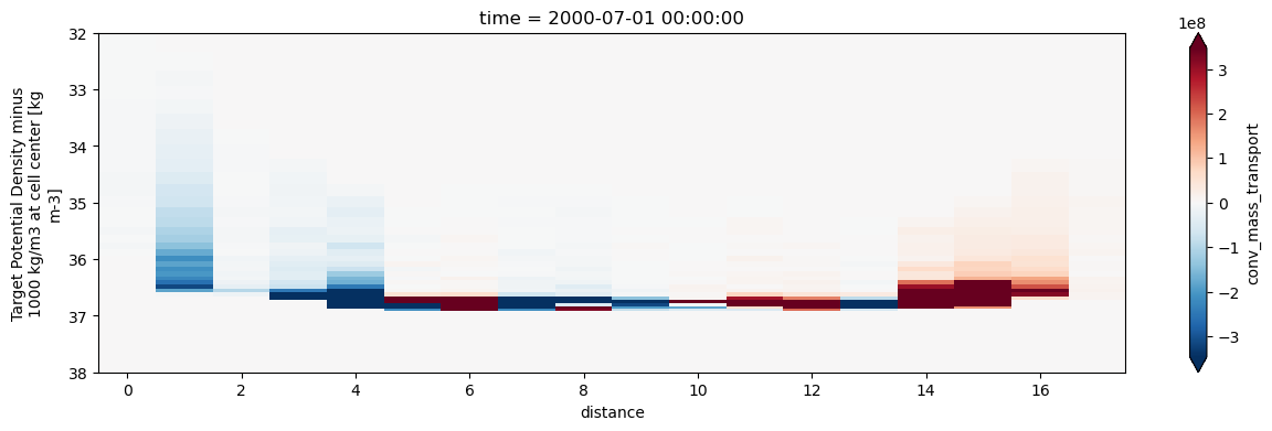
Plot cell-integrated mass transport across the section
[6]:
Trp_west = sectionate.convergent_transport(grid, i_c, j_c, layer="sigma2_l", interface="sigma2_i")
/Users/hfdrake/code/sectionate/sectionate/transports.py:393: UserWarning: The orientation of open sections is ambiguous–verify that it matches expectations!
  warnings.warn("The orientation of open sections is ambiguous–verify that it matches expectations!")
[7]:
plt.figure(figsize=(15, 4))
Trp_west.isel(time=0)['conv_mass_transport'].swap_dims({'sect':'distance'}).plot(cmap='RdBu_r', x="distance", yincrease=False, ylim=[38,32], robust=True);
Visualizing the normal vectors to understand the orientation of the cross-section transports
[8]:
plt.figure(figsize=(8.5, 3.5))
plt.pcolormesh(ds['geolon_c'], ds['geolat_c'], ds['deptho'].where(ds['deptho']!=0), vmin=0, vmax=5000, cmap="viridis_r")

plt.plot(west_section_lons, west_section_lats, "C0o", alpha=0.4)
for (p, (var, lon, lat, sign)) in enumerate(zip(
    Trp_west.dir.values,
    Trp_west.lon.values,
    Trp_west.lat.values,
    Trp_west.sign.values
    )):
    if var=="V":
        efact = 0.
        nfact = sign
    if var=="U":
        efact = sign
        nfact = 0.

    plt.annotate(
        '', xy=(lon+float(efact), lat+float(nfact)),  xycoords='data',
        xytext=(lon, lat),
        arrowprops=dict(facecolor='black', shrink=0.01, width=0.25, headwidth=5., headlength=4., alpha=0.4),
        horizontalalignment='center', verticalalignment='center'
    )
plt.plot(lons_c, lats_c, "ko-", alpha=0.5, markersize=3, label="tracer cell corners (vorticity grid)")
plt.plot(Trp_west.lon, Trp_west.lat, "C1o", alpha=0.5, lw=1, markersize=3, label="velocity cells (faces normal to section)");
plt.title("Visualizing the orientation of normal vectors")
plt.axis([-60, 0, 48, 65]);
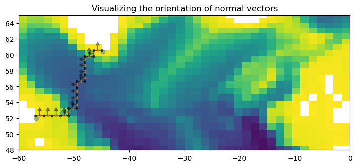
Note! We reverse the sign of the transport so that the AMOC’s deep southward transport is positive
[9]:
Trp_west = -Trp_west
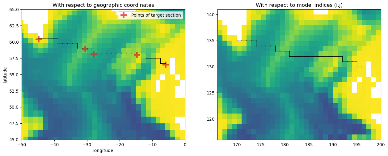
East section
[10]:
i_c, j_c, lons_c, lats_c = sectionate.grid_section(
    grid,
    east_section_lons,
    east_section_lats,
    topology="MOM-tripolar"
)
[11]:
plt.figure(figsize=[15,5.5])
plt.subplot(1,2,1)
plt.pcolormesh(ds['geolon_c'], ds['geolat_c'], ds['deptho'].where(ds['deptho']!=0), cmap="viridis_r")
plt.plot(east_section_lons, east_section_lats, "C3+", markersize=15., mew=4., alpha=0.75, label="Points of target section")
plt.plot(lons_c, lats_c, 'k.-', markersize=1.5, lw=0.75)
plt.axis([-50, 0, 45, 65])
plt.xlabel("longitude")
plt.ylabel("latitude")
plt.title("With respect to geographic coordinates")
plt.legend(loc="upper right")

plt.subplot(1,2,2)
plt.pcolormesh(ds['deptho'].where(ds['deptho']!=0), cmap="viridis_r")
plt.plot(i_c, j_c, 'k.-', markersize=1.5, lw=0.75)
plt.axis([166, 200, 116, 141])
plt.title("With respect to model indices (i,j)")
plt.show()
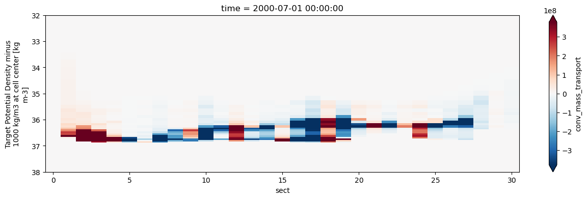
Plot the cell-integrated mass transport across the section
[12]:
Trp_east = sectionate.convergent_transport(grid, i_c, j_c, layer="sigma2_l", interface="sigma2_i")
/Users/hfdrake/code/sectionate/sectionate/transports.py:393: UserWarning: The orientation of open sections is ambiguous–verify that it matches expectations!
  warnings.warn("The orientation of open sections is ambiguous–verify that it matches expectations!")
[13]:
plt.figure(figsize=(15, 4))
Trp_east.isel(time=0)['conv_mass_transport'].plot(cmap='RdBu_r', x="sect", yincrease=False, ylim=[38,32], robust=True);
Visualizing the normal vectors to understand the orientation of the cross-section transports
[14]:
plt.figure(figsize=(8.5, 3.5))
plt.pcolormesh(ds['geolon_c'], ds['geolat_c'], ds['deptho'].where(ds['deptho']!=0), vmin=0, vmax=5000, cmap="viridis_r")

plt.plot(east_section_lons, east_section_lats, "C0o", alpha=0.4)
for (p, (var, lon, lat, sign)) in enumerate(zip(
    Trp_east.dir.values,
    Trp_east.lon.values,
    Trp_east.lat.values,
    Trp_east.sign.values
    )):
    if var=="V":
        efact = 0.
        nfact = sign
    if var=="U":
        efact = sign
        nfact = 0.

    plt.annotate(
        '', xy=(lon+float(efact), lat+float(nfact)),  xycoords='data',
        xytext=(lon, lat),
        arrowprops=dict(facecolor='black', shrink=0.01, width=0.25, headwidth=5., headlength=4., alpha=0.4),
        horizontalalignment='center', verticalalignment='center'
    )
plt.plot(lons_c, lats_c, "ko-", alpha=0.5, markersize=3, label="tracer cell corners (vorticity grid)")
plt.plot(Trp_east.lon, Trp_east.lat, "C1o", alpha=0.5, lw=1, markersize=3, label="velocity cells (faces normal to section)");
plt.title("Visualizing the orientation of normal vectors")
plt.axis([-60, 0, 48, 65]);
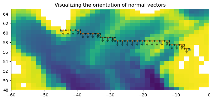
The Eastern section already has a southward orientation, so we do not need to manually flip its sign convention.
Both sections together
[15]:
i_c, j_c, lons_c, lats_c = sectionate.grid_section(
    grid,
    total_section_lons,
    total_section_lats,
    topology="MOM-tripolar"
)
[16]:
Trp = sectionate.convergent_transport(grid, i_c, j_c, layer="sigma2_l", interface="sigma2_i")
/Users/hfdrake/code/sectionate/sectionate/transports.py:393: UserWarning: The orientation of open sections is ambiguous–verify that it matches expectations!
  warnings.warn("The orientation of open sections is ambiguous–verify that it matches expectations!")
[17]:
plt.figure(figsize=(8.5, 3.5))
plt.pcolormesh(ds['geolon_c'], ds['geolat_c'], ds['deptho'].where(ds['deptho']!=0), vmin=0, vmax=5000, cmap="viridis_r")

plt.plot(total_section_lons, total_section_lats, "C0o", alpha=0.4)
for (p, (var, lon, lat, sign)) in enumerate(zip(
    Trp.dir.values,
    Trp.lon.values,
    Trp.lat.values,
    Trp.sign.values
    )):
    if var=="V":
        efact = 0.
        nfact = sign
    if var=="U":
        efact = sign
        nfact = 0.

    plt.annotate(
        '', xy=(lon+float(efact), lat+float(nfact)),  xycoords='data',
        xytext=(lon, lat),
        arrowprops=dict(facecolor='black', shrink=0.01, width=0.25, headwidth=5., headlength=4., alpha=0.4),
        horizontalalignment='center', verticalalignment='center'
    )
plt.plot(lons_c, lats_c, "ko-", alpha=0.5, markersize=3, label="tracer cell corners (vorticity grid)")
plt.plot(Trp.lon, Trp.lat, "C1o", alpha=0.5, lw=1, markersize=3, label="velocity cells (faces normal to section)");
plt.title("Visualizing the orientation of normal vectors")
plt.axis([-60, 0, 48, 65]);

Diagnosing overturning streamfunctions in density space
[18]:
rho0 = 1035. # kg/m3
Sv_s_per_m3 = 1e-6
Sv_s_per_kg = Sv_s_per_m3/rho0
ovt_rho2_west = Trp_west["conv_mass_transport"].cumsum("sigma2_l").sum("sect") *Sv_s_per_kg
ovt_rho2_east = Trp_east["conv_mass_transport"].cumsum("sigma2_l").sum("sect") *Sv_s_per_kg
ovt_rho2 = Trp["conv_mass_transport"].cumsum("sigma2_l").sum("sect") *Sv_s_per_kg
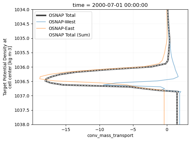
OSNAP Total Residual Transport
[19]:
(ovt_rho2).isel(time=0).plot(y='rho2_l', yincrease=False, ylim=[1038,1034], label="OSNAP Total", color="k", lw=3.5, alpha=0.75)
ovt_rho2_west.isel(time=0).plot(y='rho2_l', yincrease=False, ylim=[1038,1034], label="OSNAP-West", alpha=0.5, ls="-")
ovt_rho2_east.isel(time=0).plot(y='rho2_l', yincrease=False, ylim=[1038,1034], label="OSNAP-East", alpha=0.5, ls="-")
(ovt_rho2_east + ovt_rho2_west).isel(time=0).plot(y='rho2_l', yincrease=False, ylim=[1038,1034], label="OSNAP Total (Sum)", color="white", ls="--", lw=1.25)
plt.legend();
plt.grid(True, alpha=0.1)
[ ]: