Computing velocity-grid following sections with sectionate
In this example, we use the sectionate.grid_section function to find the indices for the series of grid cell faces (corresponding to velocity points on an Arakawa “C-grid” model such as MOM6) that best approximate a hydrographic section input by the user. In this case, we consider both the West and East sections of the Overturning of the Subpolar North Atlantic (OSNAP) observational program.
We consider both cases of MOM6’s horizontal grid configurations: non-symmetric (excluding the cell faces at the western and southern edges of the domain; also used in MOM5 and the MITgcm C-grids) and symmetric (including all tracer cell faces).
Import packages
[1]:
import xgcm
import xarray as xr
import numpy as np
import matplotlib.pylab as plt

import sectionate
print(f"Sectionate version: {sectionate.__version__}")
Sectionate version: 0.3.3
1. Unlabelled sections
A) Non-symmetric grid example (MOM5)
Load the model grid
[2]:
ds = xr.open_dataset('../data/MOM5_global_example_grid.nc')

# Sectionate requires xgcm grid objects so that it knows the model's grid metrics
# and horizontal boundary conditions.
coords={
    'X': {'center': 'xt_ocean', 'right': 'xu_ocean'},
    'Y': {'center': 'yt_ocean', 'right': 'yu_ocean'},
}
grid = xgcm.Grid(ds, coords=coords, boundary={"X":"periodic", "Y":"extend"}, autoparse_metadata=False)
display(grid)
<xgcm.Grid>
X Axis (periodic, boundary='periodic'):
  * center   xt_ocean --> right
  * right    xu_ocean --> center
Y Axis (not periodic, boundary='extend'):
  * center   yt_ocean --> right
  * right    yu_ocean --> center
Define section start, end, and some intermediate points to capture the general structure
[3]:
# Some hard-coded coordinates that approximate the OSNAP section
west_section_lons=[-56.8775, -52.0956, -49.8604, -47.6107, -44.8000]
west_section_lats=[52.0166, 52.6648, 53.5577, 58.8944, 60.4000]
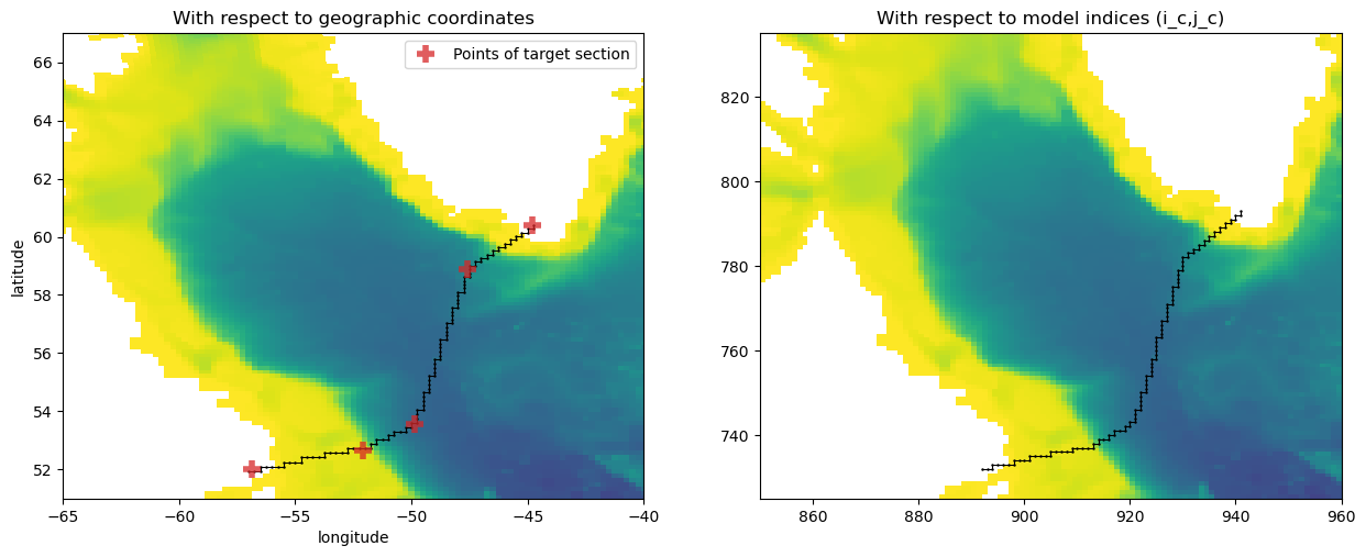
We call sectionate.grid_section to map our target section onto the model grid. Behind the scenes, sectionate.create_section_composite iterates through each of the consecutive linear segments in the section and uses sectionate.create_section to approximate them with the closest series of consecutive points on the “corner” points that corresponding to the vorticity grid (i.e. which connect the cell faces on which velocities are defined).
[4]:
i_c,j_c,lons_c,lats_c = sectionate.grid_section(
    grid,
    west_section_lons,
    west_section_lats,
    topology="MOM-tripolar"
)
[5]:
# Visualize the section in terms of both geographic coordinates and indices
plt.figure(figsize=[15,5.5])
plt.subplot(1,2,1)
plt.pcolormesh(ds['geolon_t'], ds['geolat_t'], ds['ht'][1::,1::], cmap="viridis_r")
plt.plot(lons_c, lats_c, 'k.-', markersize=1.5, lw=0.75)
plt.plot(west_section_lons, west_section_lats, "C3+", markersize=12., mew=4., alpha=0.75, label="Points of target section")
plt.axis([-65,-40, 51, 67])
plt.xlabel("longitude")
plt.ylabel("latitude")
plt.title("With respect to geographic coordinates")
plt.legend(loc="upper right")

plt.subplot(1,2,2)
plt.pcolormesh(ds['ht'].values, cmap="viridis_r")
plt.plot(i_c+1, j_c+1, 'k.-', markersize=1.5, lw=0.75) # add 1 to line up with tracer cell convention
plt.axis([850,960, 725, 835])
plt.title("With respect to model indices (i_c,j_c)")
plt.show()
Find the locations of the velocity points from the section defined by corner indices
[6]:
uvindices = sectionate.uvindices_from_qindices(grid, i_c, j_c)
lons, lats = sectionate.uvcoords_from_uvindices(
    grid,
    uvindices,
)
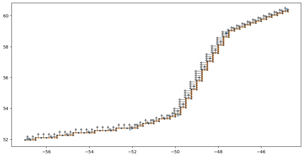
Section orientation metadata
Sectionate keeps track of the orientation of each section to ensure normal vectors have self-consistent sign conventions. The default orientation is such that a closed section will be clockwise when viewed from the south pole stereographic projection.
[7]:
plt.figure(figsize=(12, 6))
plt.plot(west_section_lons, west_section_lats, "C0o", alpha=0.4)
for (p, (var, lon, lat, nward, eward)) in enumerate(zip(uvindices['var'], lons, lats, uvindices['nward'], uvindices['eward'])):
    if var=="V":
        efact = 0.
        nfact = -1 if not(eward) else 1
    if var=="U":
        efact = -1 if nward else 1
        nfact = 0.

    plt.annotate('', xy=(lon+float(efact)*0.35, lat+float(nfact)*0.3),  xycoords='data',
            xytext=(lon, lat),
            arrowprops=dict(facecolor='black', shrink=0.01, width=0.25, headwidth=5., headlength=4., alpha=0.4),
            horizontalalignment='center', verticalalignment='center')
plt.plot(lons_c, lats_c, "ko-", alpha=0.5, markersize=3, label="tracer cell corners (vorticity grid)")
plt.plot(lons, lats, "C1o", alpha=0.5, lw=1, markersize=3, label="velocity cells (faces normal to section)");
B) Symmetric grid example (MOM6)
Download example model output and generate grid
[8]:
from load_example_model_grid import load_MOM6_example_grid
grid = load_MOM6_example_grid()
ds = grid._ds
Define section start, end, and some intermediate points to capture the general structure
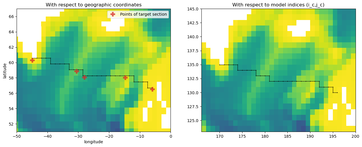
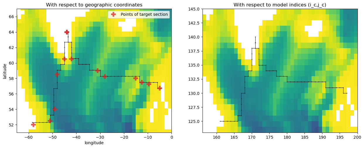
We now consider a different section, which roughly corresponds to the Eastern part of the OSNAP array.
[9]:
east_section_lats=[60.3000, 58.8600, 58.0500, 58.0000, 56.5000]
east_section_lons=[-44.9000, -30.5400, -28.0000, -14.7000, -5.9300]
We iterate on each linear segment of the section to better follow the path of the ship. We use sectionate.create_section to find the path of adjacent tracer cell indices that most closely follow each segment. The sub-sections for each linear segment are then appended to common arrays to build the full section.
Note: the last point of a segment is removed to not duplicate the first point of the following segment.
[10]:
i_c,j_c,lons_c,lats_c = sectionate.grid_section(
    grid,
    east_section_lons,
    east_section_lats,
    topology="MOM-tripolar"
)
[11]:
plt.figure(figsize=[15,5.5])
plt.subplot(1,2,1)
plt.pcolormesh(ds['geolon_c'], ds['geolat_c'], ds['deptho'].where(ds['deptho']!=0), cmap="viridis_r")
plt.plot(lons_c, lats_c, 'k.-', markersize=1.5, lw=0.75)
plt.plot(east_section_lons, east_section_lats, "C3+", markersize=12., mew=4., alpha=0.75, label="Points of target section")
plt.axis([-50, 0, 51, 67])
plt.xlabel("longitude")
plt.ylabel("latitude")
plt.title("With respect to geographic coordinates")
plt.legend(loc="upper right")

plt.subplot(1,2,2)
plt.pcolormesh(ds['deptho'].where(ds['deptho']!=0).values, cmap="viridis_r")
plt.plot(i_c, j_c, 'k.-', markersize=1.5, lw=0.75)
plt.axis([166, 200, 123, 145])
plt.title("With respect to model indices (i_c,j_c)")
plt.show()
[12]:
uvindices = sectionate.uvindices_from_qindices(grid, i_c, j_c)
lons, lats = sectionate.uvcoords_from_uvindices(
    grid,
    uvindices
)
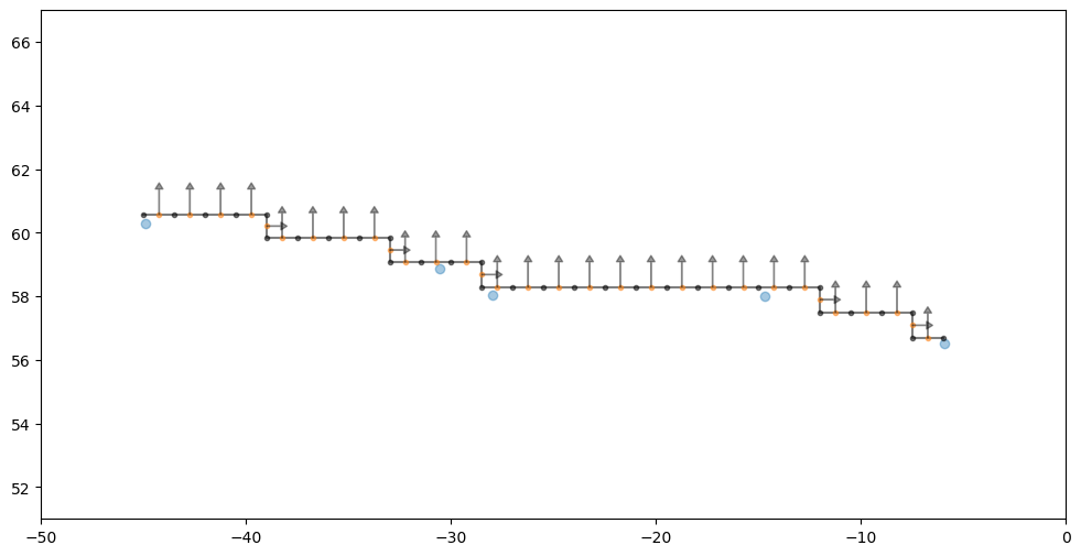
[13]:
plt.figure(figsize=(12, 6))
plt.plot(east_section_lons, east_section_lats, "C0o", alpha=0.4)
for (p, (var, lon, lat, nward, eward)) in enumerate(zip(uvindices['var'], lons, lats, uvindices['nward'], uvindices['eward'])):
    if var=="V":
        efact = 0.
        nfact = -1 if not(eward) else 1
    if var=="U":
        efact = -1 if nward else 1
        nfact = 0.

    plt.annotate('', xy=(lon+float(efact), lat+float(nfact)),  xycoords='data',
            xytext=(lon, lat),
            arrowprops=dict(facecolor='black', shrink=0.01, width=0.25, headwidth=5., headlength=4., alpha=0.4),
            horizontalalignment='center', verticalalignment='center')
plt.plot(lons_c, lats_c, "ko-", alpha=0.5, markersize=3, label="tracer cell corners (vorticity grid)")
plt.plot(lons, lats, "C1o", alpha=0.5, lw=1, markersize=3, label="velocity cells (faces normal to section)");
plt.axis([-50, 0, 51, 67])
[13]:
(np.float64(-50.0), np.float64(0.0), np.float64(51.0), np.float64(67.0))
2. Labelled Sections
When running analyses that involve many different sections and possibly multiply different model grids, it is helpful to use the labelled Section or GriddedSection classes to keep track of all the section-related data and metadata.
A) Section: named sections (with support for tracking child/parent relationships to other sections)
A Section consists of a label (or section name) coupled to the section’s coordinates:
[14]:
osnap_west = sectionate.Section(
    "OSNAP-West",
    (west_section_lons, west_section_lats)
)
display(osnap_west)

osnap_east = sectionate.Section(
    "OSNAP-East",
    (east_section_lons, east_section_lats)
)
display(osnap_east)
Section(OSNAP-West, [(-56.8775, 52.0166), (-52.0956, 52.6648), (-49.8604, 53.5577), (-47.6107, 58.8944), (-44.8, 60.4)])
attributes:
  name
  coords
  lons_c
  lats_c
  parent
Section(OSNAP-East, [(-44.9, 60.3), (-30.54, 58.86), (-28.0, 58.05), (-14.7, 58.0), (-5.93, 56.5)])
attributes:
  name
  coords
  lons_c
  lats_c
  parent
Some common sections are preset in sectionate/catalog/*.json files and can be loaded in directly without specifying their coordinates. The utils module contains various utility functions to browse the catalog. For example, the get_all_section_names function searches through the entires catalog and returns a list of the names of all available sections.
[15]:
sorted(sectionate.utils.get_all_section_names())
[15]:
['11S',
 'Bering Strait',
 'Davis Strait',
 'Denmark Strait',
 'English Channel',
 'Faroe Bank',
 'Faroe Current',
 'Fram Strait',
 'Isthmus of Panama',
 'MOVE 16N',
 'NOAC 47N',
 'OSNAP East',
 'OSNAP West',
 'Quebec',
 'RAPID 26N',
 'SAMBA',
 'Strait of Gibraltar',
 'Western Europe']
The OSNAP West and OSNAP East sections defined manually above are already available in the catalog, for example!
[16]:
osnap_west = sectionate.load_section("OSNAP West")
display(osnap_west)

osnap_east = sectionate.load_section("OSNAP East")
display(osnap_east)
Section(OSNAP West, [(-58.0, 52.0), (-51.0, 52.5), (-49.0, 54.0), (-48.0, 58.5), (-45.0, 60.5), (-44.0, 64.0)])
attributes:
  name
  coords
  lons_c
  lats_c
  parent
Section(OSNAP East, [(-44.0, 64.0), (-42.0, 60.5), (-31.0, 59.0), (-28.0, 58.25), (-15.0, 58.0), (-12.5, 57.5), (-9.5, 57.25), (-5.0, 56.75)])
attributes:
  name
  coords
  lons_c
  lats_c
  parent
A convenient property of Sections is that they can be joined together to create “parent” sections that keep track of their “child” sections.
[17]:
osnap = sectionate.join_sections("OSNAP", osnap_west, osnap_east)
display(osnap)
Section(OSNAP, [(-58.0, 52.0), (-51.0, 52.5), (-49.0, 54.0), (-48.0, 58.5), (-45.0, 60.5), (-44.0, 64.0), (-44.0, 64.0), (-42.0, 60.5), (-31.0, 59.0), (-28.0, 58.25), (-15.0, 58.0), (-12.5, 57.5), (-9.5, 57.25), (-5.0, 56.75)])
attributes:
  name
  coords
  lons_c
  lats_c
  parent
  children:
    - Section(OSNAP West, [(-58.0, 52.0), (-51.0, 52.5), (-49.0, 54.0), (-48.0, 58.5), (-45.0, 60.5), (-44.0, 64.0)])
    - Section(OSNAP East, [(-44.0, 64.0), (-42.0, 60.5), (-31.0, 59.0), (-28.0, 58.25), (-15.0, 58.0), (-12.5, 57.5), (-9.5, 57.25), (-5.0, 56.75)])
We can trace these sections along a model grid just as before:
[18]:
i_c, j_c, lons_c, lats_c = sectionate.grid_section(
    grid,
    osnap.lons_c,
    osnap.lats_c,
    topology="MOM-tripolar"
)
[19]:
plt.figure(figsize=[15,5.5])
plt.subplot(1,2,1)
plt.pcolormesh(ds['geolon_c'], ds['geolat_c'], ds['deptho'].where(ds['deptho']!=0), cmap="viridis_r")
plt.plot(lons_c, lats_c, 'k.-', markersize=1.5, lw=0.75)
plt.plot(osnap.lons_c, osnap.lats_c, "C3+", markersize=12., mew=4., alpha=0.75, label="Points of target section")
plt.axis([-65, 0, 51, 67])
plt.xlabel("longitude")
plt.ylabel("latitude")
plt.title("With respect to geographic coordinates")
plt.legend(loc="upper right")

plt.subplot(1,2,2)
plt.pcolormesh(ds['deptho'].where(ds['deptho']!=0).values, cmap="viridis_r")
plt.plot(i_c, j_c, 'k.-', markersize=1.5, lw=0.75)
plt.axis([156, 200, 123, 145])
plt.title("With respect to model indices (i_c,j_c)")
plt.show()
B) GriddedSection: grid-native named sections
A GriddedSection extends the concept of a labelled Section by coupling the Section to a specific instance of a model’s xgcm.Grid class.
[20]:
osnap_gridded = sectionate.GriddedSection(
    osnap,
    grid
)
osnap_gridded
[20]:
Section(OSNAP, [(-58.0, 52.0), (-51.0, 52.5), (-49.0, 54.0), (-48.0, 58.5), (-45.0, 60.5), (-44.0, 64.0), (-44.0, 64.0), (-42.0, 60.5), (-31.0, 59.0), (-28.0, 58.25), (-15.0, 58.0), (-12.5, 57.5), (-9.5, 57.25), (-5.0, 56.75)])
attributes:
  name
  coords
  lons_c
  lats_c
  parent
  grid
  i_c
  j_c
  children:
    - Section(OSNAP West, [(-58.0, 52.0), (-51.0, 52.5), (-49.0, 54.0), (-48.0, 58.5), (-45.0, 60.5), (-44.0, 64.0)])
    - Section(OSNAP East, [(-44.0, 64.0), (-42.0, 60.5), (-31.0, 59.0), (-28.0, 58.25), (-15.0, 58.0), (-12.5, 57.5), (-9.5, 57.25), (-5.0, 56.75)])
Since mapping sections across high-resolution grids can be a bottleneck, we also provide utilities to save and load grided datasets.
[21]:
# Saving
sectionate.utils.save_gridded_section("/tmp/osnap_gridded.json", osnap_gridded)

# Loading
osnap_gridded = sectionate.utils.load_gridded_section("/tmp/osnap_gridded.json", grid)
Finally, we revisualize the entire gridded OSNAP section.
[22]:
plt.figure(figsize=[15,5.5])
plt.subplot(1,2,1)
plt.pcolormesh(ds['geolon_c'], ds['geolat_c'], ds['deptho'].where(ds['deptho']!=0), cmap="viridis_r")
plt.plot(osnap_gridded.lons_c, osnap_gridded.lats_c, 'k.-', markersize=1.5, lw=0.75)
plt.plot(osnap.lons_c, osnap.lats_c, "C3+", markersize=12., mew=4., alpha=0.75, label="Points of target section")
plt.axis([-65, 0, 51, 67])
plt.xlabel("longitude")
plt.ylabel("latitude")
plt.title("With respect to geographic coordinates")
plt.legend(loc="upper right")

plt.subplot(1,2,2)
plt.pcolormesh(ds['deptho'].where(ds['deptho']!=0).values, cmap="viridis_r")
plt.plot(osnap_gridded.i_c, osnap_gridded.j_c, 'k.-', markersize=1.5, lw=0.75)
plt.axis([156, 200, 123, 145])
plt.title("With respect to model indices (i_c,j_c)")
plt.show()

[ ]: