Conservatively diagnosing model transports into an arbitrary closed region with sectionate

Import packages

import numpy as np
import xgcm
import xarray as xr
import matplotlib.pyplot as plt

import sectionate
print(f"Sectionate version: {sectionate.__version__}")

Sectionate version: 0.3.3

Load example model grid and transport diagnosics

from load_example_model_grid import load_MOM6_example_grid
grid = load_MOM6_example_grid()
ds = grid._ds

Define the two OSNAP sections:

Labrador_section_lons=[-56.8775, -52.0956, -49.8604, -47.6107, -44.8000, -50, -65, -65]
Labrador_section_lats=[52.0166, 52.6648, 53.5577, 58.8944, 60.4000, 71, 63.5, 57.5]
Labrador_section_lons = np.append(Labrador_section_lons, Labrador_section_lons[0])
Labrador_section_lats = np.append(Labrador_section_lats, Labrador_section_lats[0])

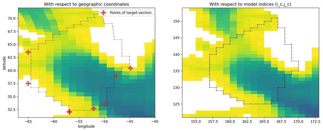
Closed section surrounding Labrador Sea

i_c, j_c, lons_c, lats_c = sectionate.grid_section(
    grid,
    Labrador_section_lons,
    Labrador_section_lats,
    topology="MOM-tripolar"
)

depth_masked = ds['deptho'].where(ds['deptho'] != 0)

plt.figure(figsize=[15,5.5])
plt.subplot(1,2,1)
plt.pcolormesh(ds['geolon_c'], ds['geolat_c'], depth_masked, cmap="viridis_r")
plt.plot(Labrador_section_lons, Labrador_section_lats, "C3+", markersize=15., mew=4., alpha=0.75, label="Points of target section")
plt.plot(lons_c, lats_c, 'k.-', markersize=1., lw=0.3)
plt.axis([-67,-40, 51, 72])
plt.xlabel("longitude")
plt.ylabel("latitude")
plt.title("With respect to geographic coordinates")
plt.legend(loc="upper right")

plt.subplot(1,2,2)
plt.pcolormesh(depth_masked, cmap="viridis_r")
plt.plot(i_c, j_c, 'k.-', markersize=1.5, lw=0.5)
plt.axis(np.array([920, 1040, 730, 925])//6)
plt.title("With respect to model indices (i_c,j_c)")
plt.show()

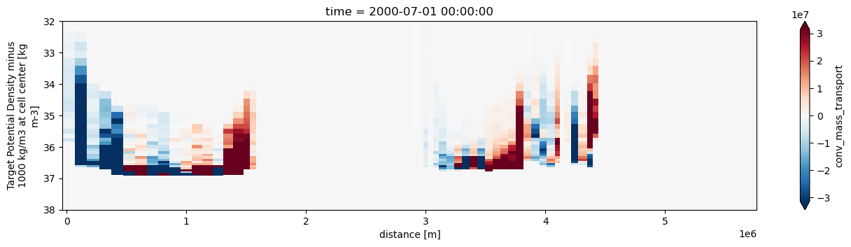
Plot the hydrography and cell-integrated mass transport across the section

T = sectionate.extract_tracer('thetao', grid, i_c, j_c)

Trp = sectionate.convergent_transport(grid, i_c, j_c, layer="sigma2_l", interface="sigma2_i")
Trp = Trp.assign_coords({"distance": xr.DataArray(Trp.dl.cumsum("sect").values, dims=("sect",), attrs={"units":"m"})})

plt.figure(figsize=(16, 3.5))
Trp.isel(time=0)['conv_mass_transport'].swap_dims({'sect':'distance'}).plot(
    cmap='RdBu_r', x="distance", yincrease=False, ylim=[38,32], robust=True
);